
Engineering Guide to Foil Strain Gauges: Working Principle, Wheatstone Bridge Topologies, and Signal ConditioningEngineering Guide to Foil Strain Gauges: Working Principle, Wheatstone Bridge Topologies, and Signal Conditioning
Foil strain gauges convert mechanical deformation into proportional electrical resistance changes via the piezoresistive effect. Standardized at nominal gauge resistances of 120 Ω or 350 Ω, metallic foil grids (typically Constantan or Karma alloy) are configured in Quarter-, Half-, or Full-Wheatstone Bridge circuits to measure microstrain (µε). Achieving high measurement precision in industrial environments requires thermal drift compensation (STC matching and 3-wire connections), 6-wire remote sensing excitation to eliminate line-resistance voltage drops, exact shunt calibration, and robust IP67/IP69K protective encapsulation.
1. Fundamental Physics & Strain Gauge Mechanics
A foil strain gauge relies on the piezoresistive effect where physical elongation or compression alters the electrical resistance of a metallic conductor. Gauge Factor (GF ≈ 2.0 for Constantan) defines sensor sensitivity, relating fractional resistance change (ΔR / R₀) directly to mechanical strain (ε = ΔL / L₀).
NOTE: To see how these fundamental foil strain gauges are integrated into physical force sensor flexures, explore our Industrial Load Cell Selection & Sourcing Guide. If your application requires high noise immunity or multi-sensor daisy chaining, read our deep-dive on Digital Load Cell Architecture & Industrial Bus Integration.
Piezoresistive Effect and Electrical Resistance Dynamics
The operation of a bonded metallic foil strain gauge is grounded in classical electrical resistance geometry:
R = ρ × (L / A)
Where:
- R = Electrical resistance (Ω)
- ρ = Resistivity of the foil material (Ω·m)
- L = Length of the conductor grid (m)
- A = Cross-sectional area of the conductor (m²)
When an external mechanical force stretches the substrate, the etched serpentine grid elongates (ΔL > 0) while Poisson contraction reduces its cross-sectional area (ΔA < 0). Both geometric changes simultaneously increase the net electrical resistance R. Conversely, compressive loading shortens the grid and increases cross-sectional area, decreasing overall resistance.
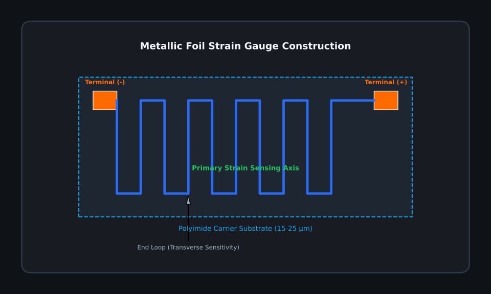
Foil Alloy Comparison: Constantan vs. Karma
- Constantan Alloy (55% Cu, 45% Ni): The industry standard for static and dynamic strain measurement. Offers a stable Gauge Factor (GF ≈ 2.0) across wide thermal windows, high fatigue life, and excellent response when matched to self-temperature-compensation (STC) substrate expansion coefficients.
- Karma Alloy (Ni-Cr-Al-Fe): Preferred for high-temperature applications (>200°C) and long-term transducer stability. Demonstrates superior fatigue resistance and lower thermal output drift, making it ideal for precision industrial load cells.
Gauge Factor (GF) and Mechanical Strain Correlation
The Gauge Factor (GF) quantifies the strain sensitivity of a sensor element:
GF = (ΔR / R₀) / ε = (ΔR / R₀) / (ΔL / L₀)
Where:
- R₀ = Nominal unstrained gauge resistance (120 Ω, 350 Ω, or 1000 Ω)
- ΔR = Resistance change induced by strain (Ω)
- ε = Mechanical strain in dimensionless units or microstrain (µε, where 1 µε = 1 × 10⁻⁶ m/m)
Transverse sensitivity (K_t) accounts for minor strain sensitivity along the end loops perpendicular to the primary axial grid. High-accuracy stress analysis requires correcting GF for K_t and Poisson ratio effects of the test specimen.
2. Wheatstone Bridge Circuit Topologies
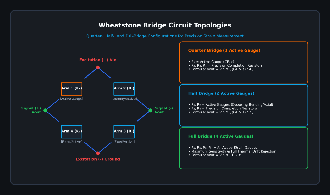
Because resistance shifts in microstrain measurements are extremely small (typically milliohms), strain gauges must be integrated into Wheatstone bridge completion circuits. Quarter-, Half-, and Full-bridge topologies convert fractional resistance variations (ΔR / R) into differential millivolt outputs (mV/V).
Quarter-Bridge Topologies (2-Wire vs. 3-Wire)
Quarter-bridge configurations utilize a single active strain gauge in Arm 1 (R₁), with three precision completion resistors forming the remaining bridge arms.
Output Voltage Equation (Quarter-Bridge):
Vout = Vin × [ (GF × ε) / 4 ]
- 2-Wire Connection Flaw: Lead-wire resistance (R_L) is in series with the active gauge. Temperature-induced resistance shifts in long lead wires create massive false strain signals (apparent thermal strain) and desensitize the gauge factor.
- 3-Wire Symmetrical Connection (Recommended): Distributes lead-wire resistance across adjacent bridge arms (R₁ and R₄). If wire resistances are equal (R_L1 = R_L2), temperature-driven lead resistance changes cancel out in the differential bridge measurement.
Half-Bridge Bending vs. Axial Topologies
Half-bridge circuits place two active gauges in the bridge (R₁ and R₂, or R₁ and R₄).
Output Voltage Equation (Half-Bridge Bending):
Vout = Vin × [ (GF × ε) / 2 ]
- Bending Strain Isolation: Active gauges mounted on opposite sides of a cantilever beam experience equal and opposite strains (ε₁ = +ε, ε₂ = -ε). Wiring them into adjacent arms doubles the output signal while automatically canceling common-mode axial strain and thermal expansion.
- Axial Poisson Configuration: One gauge aligns axially (ε₁ = ε) while the second aligns transversely (ε₂ = -ν · ε). Yields an output of Vout = Vin × [ (GF × ε × (1 + ν)) / 4 ].
Full-Bridge Configurations (Tension, Compression, Torsion)
Full-bridge configurations employ active strain gauges in all four arms (R₁, R₂, R₃, R₄).
Output Voltage Equation (Full-Bridge Bending/Tension):
Vout = Vin × GF × ε
Full-bridge topologies deliver maximum signal output (4x sensitivity compared to quarter-bridge), complete common-mode noise rejection, and superior thermal stability. They form the core architecture of commercial force sensors.
| Topology | Active Gauges | Output Sensitivity (Vout / Vin) | Thermal Self-Compensation | Primary Application |
|---|---|---|---|---|
| Quarter-Bridge Type I (2-Wire) | 1 | (1/4) × GF × ε | Poor (Requires Dummy) | Basic laboratory testing |
| Quarter-Bridge Type II (3-Wire) | 1 | (1/4) × GF × ε | Good (Lead-wire canceled) | Structural field monitoring |
| Half-Bridge Bending | 2 | (1/2) × GF × ε | Excellent | Beam deflection & shaft bending |
| Full-Bridge Transducer | 4 | GF × ε | Optimal | Precision load cells & torque sensors |
3. Thermal Drift & Environmental Compensation
Temperature fluctuations alter both the resistance of the grid alloy and the dimensions of the structural substrate, causing apparent thermal strain. Mitigating thermal drift requires Self-Temperature-Compensated (STC) alloy matching, active-dummy bridge legs, or software polynomial corrections.
Self-Temperature-Compensated (STC) Gauges
- STC Code 06: Matched to Ferritic Steel (10.8 µε/°C or 11 ppm/°C).
- STC Code 13: Matched to Aluminum Alloys (23.4 µε/°C or 23 ppm/°C).
- STC Code 29: Matched to Titanium Alloys (8.5 µε/°C).
Active-Dummy Bridge & Digital Polynomial Correction
When STC matching is insufficient under extreme thermal gradients, engineers install an unstrained dummy gauge on an identical, un-loaded block of the same metal subjected to the same thermal environment. Placed in arm R₂ of a quarter bridge, the dummy gauge cancels temperature-induced resistance changes.
In digital DAQ systems, apparent strain (εₜ) is calculated using a 3rd-order polynomial lookup table:
εₜ = A₀ + A₁T + A₂T² + A₃T³
Where T is temperature in °C and Aₙ are manufacturer gauge-lot specific calibration coefficients.
4. Signal Conditioning & Data Acquisition Architecture
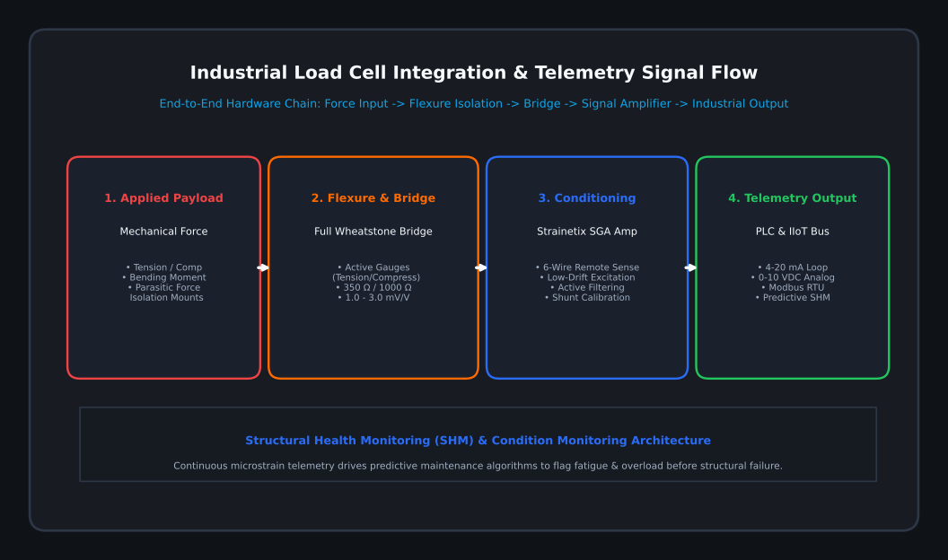
Raw millivolt bridge outputs require regulated excitation, 6-wire sense leads, differential instrumentation amplification, and active filtering to convert microstrain signals into industrial 4–20mA current loops or Modbus RTU telemetry.
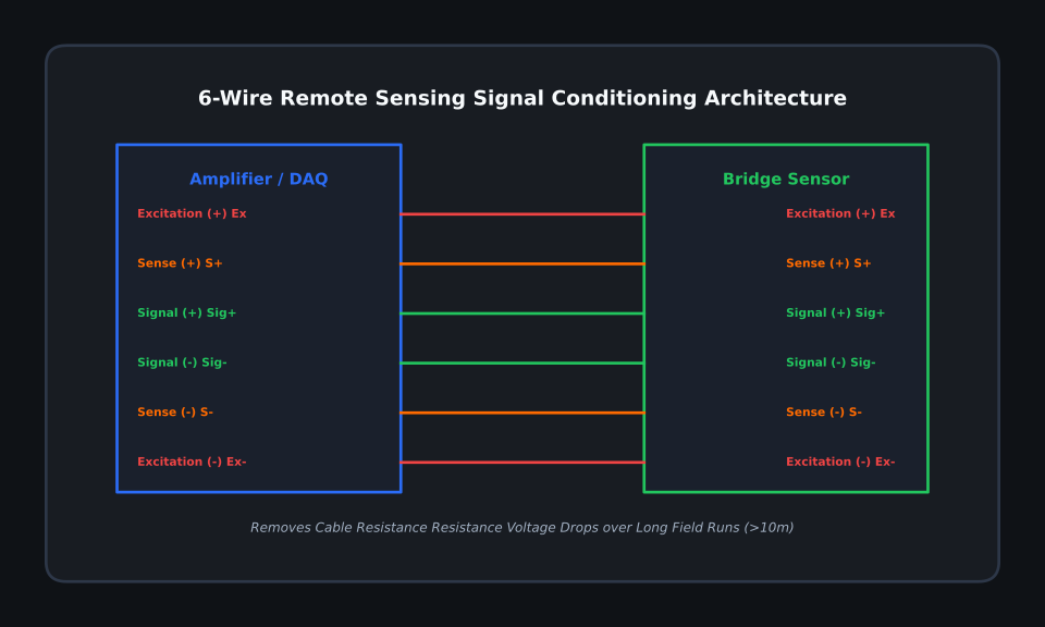
Excitation Regulation & Remote Sensing (4-Wire vs. 6-Wire)
- 4-Wire Connections: Current flow over long cable runs causes I·R voltage drops along the excitation wires, reducing voltage at the bridge terminals and creating linear gain errors.
- 6-Wire Remote Sensing: Employs two dedicated high-impedance sense leads that measure exact excitation voltage at the sensor bridge node. The signal conditioning amplifier continuously adjusts excitation drive to compensate for cable resistance drops automatically.
Bridge Balancing, Shunt Calibration, and Amplification
Shunt calibration simulates a known mechanical strain by switching a precision high-value resistor (R_s) in parallel across one arm (R_g) of the Wheatstone bridge:
R_s = [ R_g / (2 × ΔR_R) ] – (R_g / 2) = [ R_g / (GF × ε_sim) ] – (R_g / 2)
Where ε_sim is the simulated microstrain value.
Differential instrumentation amplifiers amplify the resulting 1–3 mV/V bridge output into high-level industrial signals (0–10 VDC or 4–20 mA current loops).
5. Surface Preparation, Bonding, and Environmental Protection
Measurement integrity relies entirely on bond line quality. Proper surface preparation follows a strict sequence: solvent degreasing, grit abrading, surface conditioning/neutralizing, adhesive curing, and IP67/IP69K encapsulation.
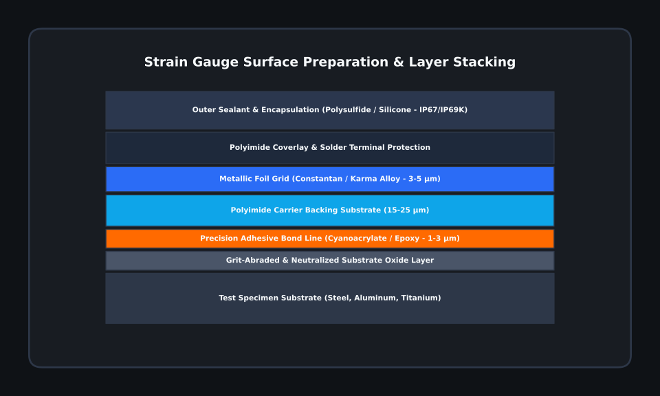
Substrate Preparation & Alignment Procedure
- Degreasing: Clean the specimen surface using mild solvent degreasers (isopropanol or acetone) to eliminate oils.
- Grit Abrading: Wet-abrade with 220 to 400 grit silicon-carbide paper to establish a cross-hatched surface roughness (R_a ≈ 1.6–3.2 µm).
- Layout Line Marking: Scribe burnished alignment marks using a soft graphite pencil or brass scribe.
- Conditioning & Neutralizing: Apply chemical conditioners to clean the abraded cross-hatches, followed by a surface neutralizer to raise pH to 7.0–7.5.
Adhesive Selection Regimes
| Adhesive Type | Temperature Range | Curing Profile | Operational Characteristics |
|---|---|---|---|
| Cyanoacrylate (Cold Curing) | -32°C to +65°C | 1–5 minutes under thumb pressure | Ideal for short-term testing & rapid prototyping. Susceptible to moisture degradation. |
| Two-Part Epoxy (Heat Curing) | -269°C to +260°C | 100–175°C for 1–4 hours | High precision, low creep, minimal hysteresis. Essential for industrial transducers. |
| Ceramic Cement | -269°C to +800°C | Multi-stage heat cure up to 300°C | Specialized for ultra-high-temperature turbine testing and nuclear applications. |
Environmental Protection & Waterproofing
Unprotected strain gauges degrade rapidly when exposed to humidity or chemicals due to insulation resistance breakdown between the grid and substrate.
- IP65/IP67 Coatings: Polyurethane overcoats backed by nitrile rubber or microcrystalline wax.
- IP69K Submersible Protection: Polysulfide sealers topped with stainless-steel shim caps and chemical-resistant silicone encapsulants for washdown environments.
6. Strain Gauge Geometries & Specialized Topologies
Selecting the correct grid geometry resolves complex stress vectors. Linear gauges measure uniaxial strain, rosettes determine principal stress directions, and diaphragm gauges measure radial deflection in pressure sensors.
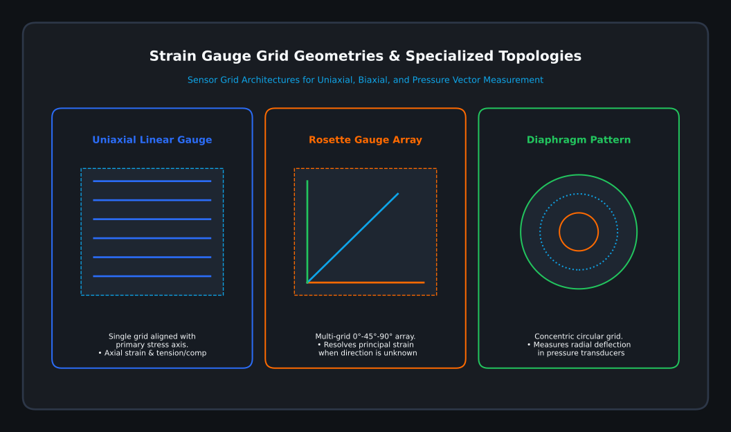
- Linear Strain Gauges: Single serpentine grid aligned along the primary stress axis.
- Rosette Strain Gauges: Multi-grid arrays (0°-45°-90° rectangular or 0°-60°-120° delta) used when principal stress directions are unknown.
- Tee Rosettes (0°-90°): Two orthogonal grids for biaxial tensile/compressive strain isolation.
- Diaphragm Strain Gauges: Concentric circular and radial grids designed for pressure sensor diaphragms.
7. Industrial Load Cells & Condition Monitoring
Bonded foil gauges serve as the primary sensing elements within industrial force sensors, torque transducers, and Structural Health Monitoring (SHM) IIoT networks.
8. Technical Troubleshooting FAQ
Q1: What causes excessive zero-drift in a freshly bonded strain gauge?
Answer: Zero-drift is most commonly caused by incomplete adhesive curing, moisture ingress causing insulation breakdown (<500 MΩ to ground), or uncompensated thermal gradient effects. Verify ground insulation resistance using a low-voltage megohmmeter.
Q2: Why is 3-wire quarter-bridge wiring preferred over 2-wire setups?
Answer: In a 2-wire setup, lead-wire resistance adds directly to the active gauge arm. Any temperature change along the cable alters lead resistance, producing apparent strain errors. A 3-wire setup places equal lead resistance in adjacent bridge arms, causing thermal resistance changes to cancel out.
Q3: How do 6-wire sense circuits eliminate long cable excitation drops?
Answer: 6-wire configurations route two dedicated high-impedance sense lines directly to the sensor bridge nodes. The amplifier measures exact bridge voltage and adjusts excitation output to eliminate cable resistance voltage drops.